< User talk:Paul WormerRevision as of 02:44, 31 March 2010 by imported>Paul Wormer
PD Image Equation for plane. X is arbitary point in plane;
and
are collinear.
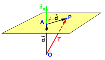
In analytic geometry several closely related algebraic equations are known for a plane in three-dimensional Euclidean space. One such equation is illustrated in the figure. Point P is an arbitrary point in the plane and O (the origin) is outside the plane. The point A in the plane is chosen such that vector
![{\displaystyle {\vec {d}}\equiv {\overrightarrow {OA}}}](https://wikimedia.org/api/rest_v1/media/math/render/svg/e36e2b3dc5fa9a5197f9893441a4d25e86c6b93c)
is orthogonal to the plane. The collinear vector
![{\displaystyle {\vec {n}}_{0}\equiv {\frac {1}{d}}{\vec {d}}\quad {\hbox{with}}\quad d\equiv \left|{\vec {d}}\,\right|}](https://wikimedia.org/api/rest_v1/media/math/render/svg/7a7618570d19e424b5ccd749b18cae10c4371922)
is a unit (length 1) vector normal (perpendicular) to the plane. Evidently d is the distance of O to the plane. The following relation holds for an arbitrary point P in the plane
![{\displaystyle \left({\vec {r}}-{\vec {d}}\;\right)\cdot {\vec {n}}_{0}=0\quad {\hbox{with}}\quad {\vec {r}}\equiv {\overrightarrow {OP}}\quad {\hbox{and}}\quad {\vec {r}}-{\vec {d}}={\overrightarrow {AP}}.}](https://wikimedia.org/api/rest_v1/media/math/render/svg/cb0fff5fff9086e57152477a370256bde96a5c85)
This equation for the plane can be rewritten in terms of coordinates with respect to a Cartesian frame with origin in O. Dropping arrows for component vectors (real triplets) that are written bold, we find
![{\displaystyle \left(\mathbf {r} -\mathbf {d} \right)\cdot \mathbf {n} _{0}=0\Longleftrightarrow xa_{0}+yb_{0}+zc_{0}=d}](https://wikimedia.org/api/rest_v1/media/math/render/svg/3d37bdf09641d6244e5f46505c76e06955934181)
with
![{\displaystyle \mathbf {d} =(a,\;b,\;c),\quad \mathbf {n} _{0}=(a_{0},\;b_{0},\;c_{0}),\quad \mathbf {r} =(x,\;y,\;z),}](https://wikimedia.org/api/rest_v1/media/math/render/svg/9795ec78f4905c32c8838372d2b23b017b6be2aa)
and
![{\displaystyle \mathbf {d} \cdot \mathbf {n} _{0}={\frac {1}{d}}\mathbf {d} \cdot \mathbf {d} =d={\sqrt {a^{2}+b^{2}+c^{2}}}.}](https://wikimedia.org/api/rest_v1/media/math/render/svg/f8561f6154d6c3187ff09f5923e8695531bef1b7)
Conversely, given the following equation for a plane
![{\displaystyle ax+by+cz=e,\,}](https://wikimedia.org/api/rest_v1/media/math/render/svg/1a29e27177c9158decab6630e79da7a59ce69b14)
it is easy to derive the same equation.
Write
![{\displaystyle \mathbf {r} =(x,\;y,\;z),\quad \mathbf {f} =(a,\;b,\;c),\quad {\hbox{and}}\quad \mathbf {d} \equiv \left({\frac {e}{a^{2}+b^{2}+c^{2}}}\right)\mathbf {f} .}](https://wikimedia.org/api/rest_v1/media/math/render/svg/7bd6bde0291ba8fd745dd5e817aa0284c087bfd7)
It follows that
![{\displaystyle \mathbf {f} \cdot \mathbf {r} =e=\mathbf {f} \cdot \mathbf {d} .}](https://wikimedia.org/api/rest_v1/media/math/render/svg/f68855edc01b123d5f3955fdf254dcb50d4d0bce)
Hence we find the same equation,
![{\displaystyle \mathbf {f} \cdot (\mathbf {r} -\mathbf {d} )=0\;\Longrightarrow \;(\mathbf {r} -\mathbf {d} )\cdot \mathbf {n} _{0}=0\quad {\hbox{with}}\quad \mathbf {n} _{0}={\frac {1}{\sqrt {a^{2}+b^{2}+c^{2}}}}\mathbf {f} }](https://wikimedia.org/api/rest_v1/media/math/render/svg/cf4ed176eb8568ce408fdbd68872ef0d739f19a5)
where f , d, and n0 are collinear. The equation may also be written in the following mnemonically convenient form
![{\displaystyle \mathbf {d} \cdot (\mathbf {r} -\mathbf {d} )=0,}](https://wikimedia.org/api/rest_v1/media/math/render/svg/55fc00923067395b6e403232526b3a0045b038f7)
which is the equation for a plane through a point A perpendicular to
.