Template:Under construction
Fixed point  of a functor
  is solution of equation
- (1)
![{\displaystyle F[L]=L}](https://wikimedia.org/api/rest_v1/media/math/render/svg/952aaf5e42e45721926eb1deb75cdc9613a87971)
Simple examples
Elementary functions
In particular, functor can be elementaty function. For example, 0 and 1 are fixed points of function sqrt, because  and
and
 .
.
In similar way, 0 is fixed point of sine function, because  .
.
Operators
Functor in the equation (1) can be a linear operator. In this case, the fixed point of functor is its eigenfunction with eigenvalue equal to unity.
Exponential if fixed point or operator of differentiation D,
because

The Gaussian exponential
- (2)
 ,
,  reals
reals
is fixed point of the Fourier operator, defined with its action on a function  :
:
- (3)

in general, functors have no need to be linear, so, there is no associativity
at application of several functors in row, and parenthesis are necessary in the left hand side of eapression (3).
[1]
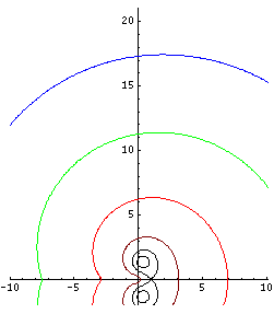
FIg.1.

is shown with levels

,

,

,

,

,

in the complex

-plane

Fig.1. The same as FIg.1 for function

Fixed points can be searched graphically. Fig.1 shows the graphical search of fixed points of logarithm,
i.e., soluitons of the equaiton
- (10)

There are no real solutions fot this equation, but there are two complex-congjugated solutions
 and
and  . However, the value of cannot be estimated well from the figure (1), but the straigtgorward iteration allows the precise estimate. Few hundreds of iterations are sufficient to get error of order of last significant figure in the
approximation
. However, the value of cannot be estimated well from the figure (1), but the straigtgorward iteration allows the precise estimate. Few hundreds of iterations are sufficient to get error of order of last significant figure in the
approximation
- (11)

Fixed points of logarithm should not be confised with fixed points of exponential, shown in FIgure 2.
Therse fixed points are solutions of equaitons
- (12)

They can be expressed also as solution of equation
- (13)
 for some integer
For example, at 
- (13)

is fixed point of the exponential, but is not the fixed point of natural logarithm.
In the case of exponential and natural logarithm, all fixed points are complex.
However,  the real fixed points exist at
  .
For example, at
.
For example, at  , number e is fixed point of both,
and
, number e is fixed point of both,
and  ; and at
  , numbers
2 and 4 are their fixed points.
, numbers
2 and 4 are their fixed points.
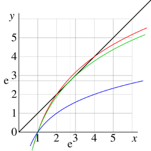
FIg.3. Example of graphic solution of equation

for
(two real solutions,

and

),

(one real solution

)

(no real solutions).
Finding of real fixed points is presented graphically in Figure 3. The black curve represents the identical function  in the left hand side of equation
- (14)

the colored curves represent the function in the right hand side for
 . In the last case, there are no real solutions, but the complex fixed points are complex numbers
  and
and  . Within few hundred iterations of equation (14), they can be approcimated with many decimal digits;
- (15)
 .
.
Tetration
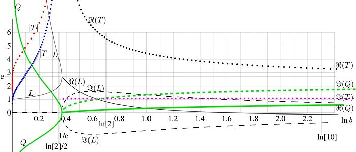
FIg.4. parameters of asymptotic of tetration versus logarithm of the base
The fixed points of logarithm determine the asymptotic properties of analytic extension of tetration  . In some range of the
complex
. In some range of the
complex  -plane, the tetration can be approximated with asymptotic
(32) 
where
(33)  ,
,
 and
and  are fixed complex numbers, dependent on
  are shown with thin black curves versus logarithm on base </math>b</math>.
At
are shown with thin black curves versus logarithm on base </math>b</math>.
At  , the fixed points are complex; the real part is shown with solid curve, the imaginary part is shown with dashed curve.
Green curves in FIgure 4 represent the parameter in (33), again, the dased curve shows the imaginary part, and
real and imaginary parts of the asymptotic period  . See article tetration for details.
Notes
- ↑
Note that that there is certain ambiguity in commonly used writing of mathematical formulas, omiting sign * of multiplication; in equation (3), expression
 does not mean that
  is multiplied to value of
  ; it means that result of action of operator on function , whith is also function, is evaluated at argument .


