imported>Anthony.Sebastian |
imported>Anthony.Sebastian |
| Line 1: |
Line 1: |
| '''Osteoporosis''' | | '''Osteoporosis''' |
|
| |
| Surgeon General (Smith 2000) <ref>Quite a guy!</ref>
| |
|
| |
| ==oiu==
| |
| Mathematics, biology’s next microscope
| |
|
| |
| :''About this article:''<ref>This article represents a permissible adaption and modification of an article by Joel E. Cohen of Rockefeller University published in the open-access journal, PLoS Biology 1(12):e439 in n2004, under the full title: [http://dx.doi.org/10.1371/journal.pbio.0020439 Mathematics is biology’s next microscope, only better; biology is mathematics’ next physics, only better.]
| |
| *Cohen JE (2004) Mathematics is biology’s next microscope, only better; biology is mathematics’ next physics, only better. PLoS Biol 2(12): e439.
| |
| *Copyright: © 2004 Joel E. Cohen. This is an open- access article distributed under the terms of the Creative Commons Attribution License, which permits unrestricted use, distribution, and reproduction in any medium, provided the original work is properly cited.
| |
| *Joel E. Cohen is at the Laboratory of Populations, Rockefeller and Columbia Universities, New York, New York, United States of America. E-mail: cohen@rockefeller.edu.
| |
| *In the original PLoS Biology article, Dr. Cohen offered the following acknowledgements:
| |
| :* This paper is based is on a talk [by Dr. Joel Cohen] given on February 12, 2003, as the keynote address at the National Science Foundation (NSF)–National Institutes of Health (NIH) Joint Symposium on Accelerating Mathematical–Biological Linkages, Bethesda, Maryland; on June 12, 2003, as the first presentation in the 21st Century Biology Lecture Series, National Science Foundation, Arlington, Virginia; and on July 10, 2003, at a Congressional Lunch Briefing, co-sponsored by the American Mathematical Society and Congressman Vernon J. Ehlers, Washington, D.C. Dt. Cohen thank Margaret Palmer, Sam Scheiner, Michael Steuerwalt, James Cassatt, Mike Marron, John Whitmarsh, and directors of NSF and NIH for organizing the NSF–NIH meeting, Mary Clutter and Joann P. Roskoski for organizing my presentation at the NSF, Samuel M. Rankin III for organizing the American Mathematical Society Congressional Lunch Briefi ng, and Congressman Bob Filner for attending and participating. Dr. Cohen expresses gratitude for constructive editing by Philip Bernstein, helpful suggestions on earlier versions from Mary Clutter, Charles Delwiche, Bruce A. Fuchs, Yonatan Grad, Alan Hastings, Kevin Lauderdale, Zaida Luthey-Schulten, Daniel C. Reuman, Noah Rosenberg, Michael Pearson, and Samuel Scheiner, support from U.S. NSF grant DEB 9981552, the help of Kathe Rogerson, and the hospitality of Mr. and Mrs. William T. Golden during this work. Any opinions, findings, and conclusions or recommendations expressed in this material do not necessarily reflect the views of the NSF.
| |
| *Article reformatted to correspond to Citizendium style, with Editor explanatory interpolations in square brackets, and a few editorial notes in References section, by Citizendium Biology Editor Anthony.Sebastian("A.S")</ref>
| |
|
| |
|
| |
| Although mathematics has long been intertwined with the biological sciences, an explosive synergy between biology and mathematics seems poised to enrich and extend both fields greatly in the coming decades (Levin 1992; Murray 1993; Jungck 1997; Hastings et al. 2003; Palmer et al. 2003; Hastings and Palmer 2003). Biology will increasingly stimulate the creation of qualitatively new realms of mathematics. Why?
| |
|
| |
| In biology, ensemble properties emerge at each level of organization from the interactions of heterogeneous biological units at that level and at lower and higher levels of organization (larger and smaller physical scales, faster and slower temporal scales). New mathematics will be required to cope with these ensemble properties and with the heterogeneity of the biological units that compose ensembles at each level.
| |
| <br>
| |
| __TOC__
| |
| <br>
| |
| ==How the discovery of the microscope challenged biology==
| |
|
| |
| The discovery of the microscope in the late 17th century caused a revolution in biology by revealing otherwise invisible and previously unsuspected worlds. Western cosmology from classical times through the end of the Renaissance envisioned a system with three types of spheres: the sphere of man, exemplified by his imperfectly round head; the sphere of the world, exemplified by the imperfectly spherical earth; and the eight perfect spheres of the universe, in which the seven (then known) planets moved and the outer stars were fixed (Nicolson 1960). The discovery of a microbial world too small to be seen by the naked eye challenged the completeness of this cosmology and unequivocally demonstrated the existence of living creatures unknown to the Scriptures of Old World religions.
| |
|
| |
| ==Mathematics as microscope==
| |
|
| |
| Mathematics broadly interpreted is a more general microscope. It can reveal otherwise invisible worlds in all kinds of data, not only optical. For example, computed tomography can reveal a cross-section of a human head from the density of X-ray beams without ever opening the head, by using the Radon transform to infer the densities of materials at each location within the head (Hsieh 2003). Charles Darwin was right when he wrote that people with an understanding “of the great leading principles of mathematics... seem to have an extra sense” (F. Darwin 1905). Today’s biologists increasingly recognize that appropriate mathematics can help interpret any kind of data. In this sense, mathematics is biology’s next microscope, only better.
| |
|
| |
| <blockquote>
| |
| <p style="color: #660000; font-size: 1.0em"><i>Mathematics broadly interpreted is a more general microscope. It can reveal otherwise invisible worlds in all kinds of data, not only optical. For example, computed tomography can reveal a cross-section of a human head from the density of X-ray beams without ever opening the head, by using the Radon transform to infer the densities of materials at each location within the head (Hsieh 2003). Charles Darwin was right when he wrote that people with an understanding “of the great leading principles of mathematics... seem to have an extra sense” (F. Darwin 1905). Today’s biologists increasingly recognize that appropriate mathematics can help interpret any kind of data. In this sense, mathematics is biology’s next microscope, only better.</i><ref>xxx</ref></p></blockquote>
| |
|
| |
|
| |
| <references/>
| |
|
| |
| ==Role of biology in the development of mathematics==
| |
|
| |
| Conversely, mathematics will benefit increasingly from its involvement with biology, just as mathematics has already benefited and will continue to benefit from its historic involvement with physical problems. In classical times, physics, as first an applied then a basic science, stimulated enormous advances in mathematics. For example, geometry reveals by its very etymology (geometry) its origin in the needs to survey the lands and waters of Earth. Geometry was used to lay out fields in Egypt after the flooding of the Nile, to aid navigation, to aid city planning. The inventions of the calculus by Isaac Newton and Gottfried Leibniz in the later 17th century were stimulated by physical problems such as planetary orbits and optical calculations.
| |
|
| |
| In the coming century, biology will stimulate the creation of entirely new realms of mathematics. In this sense, biology is mathematics’ next physics, only better. Biology will stimulate fundamentally new mathematics because living nature is qualitatively more heterogeneous than non-living nature. For example, it is estimated that there are 2,000–5,000 species of rocks and minerals in the earth’s crust, generated from the hundred or so naturally occurring elements (Shipman et al. 2003; chapter 21 estimates 2,000 minerals in Earth’s crust). By contrast, there are probably between 3 million and 100 million biological species on Earth, generated from a small fraction of the naturally occurring elements. If species of rocks and minerals may validly be compared with species of living organisms, the living world has at least a thousand times the diversity of the non-living. This comparison omits the enormous evolutionary importance of individual variability within species. Coping with the hyper-diversity of life at every scale of spatial and temporal organization will require fundamental conceptual advances in mathematics.
| |
|
| |
| ==The past interactions between mathematics and biology==
| |
|
| |
| ===William Harvey introduce ‘off-the-shelf’ mathematic into biology===
| |
|
| |
| The interactions between mathematics and biology at present follow from their interactions over the last half millennium. The discovery of the New World by Europeans approximately 500 years ago—and of its many biological species not described in religious Scriptures—gave impetus to major conceptual progress in biology.
| |
|
| |
| The outstanding milestone in the early history of biological quantitation was the work of William Harvey, Exercitatio Anatomica De Motu Cordis et Sanguinis In Animalibus (An Anatomical Disquisition on the Motion of the Heart and Blood in Animals) (Harvey 1847) [generally referred to as De Motu Cordis], first published in 1628. Harvey’s demonstration that the blood circulates was the pivotal founding event of the modern interaction between mathematics and biology. His elegant reasoning is worth understanding.
| |
|
| |
| From the time of the ancient Greek physician Galen (131–201 C.E.) until William Harvey studied medicine in Padua (1600–1602, while Galileo was active there), it was believed that there were two kinds of blood, arterial blood and venous blood. Both kinds of blood were believed to ebb and flow under the motive power of the liver, just as the tides of the earth ebbed and flowed under the motive power of the moon. Harvey became physician to the king of England. He used his position of privilege to dissect deer from the king’s deer park as well as executed criminals. Harvey observed that the veins in the human arm have one-way valves that permit blood to flow from the periphery toward the heart but not in the reverse direction. Hence the theory that the blood ebbs and flows in both veins and arteries could not be correct.
| |
|
| |
| Harvey also observed that the heart was a contractile muscle with one- way valves between the chambers on each side. He measured the volume of the left ventricle of dead human hearts and found that it held about two ounces (about 60 ml), varying from 1.5 to three ounces in different individuals. He estimated that at least one-eighth and perhaps as much as one-quarter of the blood in the left ventricle was expelled with each stroke of the heart. He measured that the heart beat 60–1 00 times per minute. Therefore, the volume of blood expelled from the left ventricle per hour was about 60 ml × 1/8 × 60 beats/minute × 60 minutes/hour, or 27 liters/hour. However, the average human has only 5.5 liters of blood (a quantity that could be estimated by draining a cadaver). Therefore, the blood must be like a stage army that marches off one side of the stage, returns behind the scenes, and reenters from the other side of the stage, again and again. The large volume of blood pumped per hour could not possibly be accounted for by the then-prevalent theory that the blood originated from the consumption of food.
| |
|
| |
| Harvey inferred that there must be some small vessels that conveyed the blood from the outgoing arteries to the returning veins, but he was not able to see those small vessels. His theoretical prediction, based on his meticulous anatomical observations and his mathematical calculations, was spectacularly confirmed more than half a century later when Marcello Malpighi (1628–1694) saw the capillaries under a microscope.
| |
|
| |
| Harvey’s discovery illustrates the enormous power of simple, off-the-shelf mathematics combined with careful observation and clear reasoning. It set a high standard for all later uses of mathematics in biology.
| |
|
| |
| ===Mendel’s mathematics and the discovery of genes===
| |
|
| |
| Mathematics was crucial in the discovery of genes by Mendel (Orel 1984) and in the theory of evolution.
| |
|
| |
| Mathematics was and continues to be the principal means of integrating evolution and genetics since the classic work of R. A. Fisher, J. B. S. Haldane, and S. Wright in the first half of the 20th century (Provine 2001).
| |
| ===The enrichment of biology by mathematical progress in geometry, topology, algebra, and analysis===
| |
|
| |
| Over the last 500 years, mathematics has made amazing progress in each of its three major fields: geometry and topology, algebra, and analysis. This progress has enriched all the biological sciences.
| |
|
| |
| In 1637, René Descartes linked the featureless plane of Greek geometry to the symbols and formulas of Arabic algebra by imposing a coordinate system (conventionally, a horizontal x-axis and a vertical y-axis) on the geometric plane and using numbers to measure distances between points. If every biologist who plotted data on x–y coordinates acknowledged the contribution of Descartes to biological understanding, the key role of mathematics in biology would be uncontested.
| |
|
| |
| Another highlight of the last five centuries of geometry was the invention of non-Euclidean geometries (1823–1830). Shocking at first, these geometries unshackled the possibilities of mathematical reasoning from the intuitive perception of space. These non-Euclidean geometries have made significant contributions to biology in facilitating, for example, mapping the brain onto a fl at surface (Hurdal et al. 1999; Bowers and Hurdal 2003).
| |
|
| |
| In algebra, efforts to find the roots of equations led to the discovery of the symmetries of roots of equations and thence to the invention of group theory, which finds routine application in the study of crystallographic groups by structural biologists today. Generalizations of single linear equations to families of simultaneous multi-variable linear equations stimulated the development of linear algebra and the European re-invention and naming of matrices in the mid- 19th century. The use of a matrix of numbers to solve simultaneous systems of linear equations can be traced back in Chinese mathematics to the period from 300 B.C.E. to 200 C.E. (in a work by Chiu Chang Suan Shu called Nine Chapters of the Mathematical Art; Smoller 2001). In the 19th century, matrices were considered the epitome of useless mathematical abstraction. Then, in the 20th century, it was discovered, for example, that the numerical processes required for the cohort-component method of population projection can be conveniently summarized and executed using matrices (Keyfi tz 1968). Today the use of matrices is routine in agencies responsible for making official population projections as well as in population-biological research on human and nonhuman populations (Caswell 2001).
| |
|
| |
| Finally, analysis, including the calculus of Newton and Leibniz and probability theory, is the line between ancient thought and modern thought. Without an understanding of the concepts of analysis, especially the concept of a limit, it is not possible to grasp much of modern science, technology, or economic theory. Those who understand the calculus, ordinary and partial differential equations, and probability theory have a way of seeing and understanding the world, including the biological world, that is unavailable to those who do not.
| |
|
| |
| ==Biology enriches mathematics==
| |
|
| |
| Conceptual and scientific challenges from biology have enriched mathematics by leading to innovative thought about new kinds of mathematics. Table 1 lists examples of new and useful mathematics arising from problems in the life sciences broadly construed, including biology and some social sciences. Many of these developments blend smoothly into their antecedents and later elaborations. For example, game theory has a history before the work of John von Neumann (von Neumann 1959; von Neumann and Morgenstern 1953), and Karl Pearson’s development of the correlation coefficient (Pearson and Lee 1903) rested on earlier work by Francis Galton (1889).
| |
|
| |
| ==Present and future interactions of mathematics and biology==
| |
|
| |
| To see how the interactions of biology and mathematics may proceed in the future, it is helpful to map the present landscapes of biology and applied mathematics.
| |
|
| |
| The biological landscape may be mapped as a rectangular table with different rows for different questions and different columns for different biological domains. Biology asks six kinds of questions.
| |
|
| |
| *How is it built?
| |
| *How does it work?
| |
| *What goes wrong?
| |
| *How is it fixed?
| |
| *How did it begin?
| |
| *What is it for?
| |
|
| |
| Those are questions, respectively, about structures, mechanisms, pathologies, repairs, origins, and functions or purposes. The former teleological interpretation of purpose has been replaced by an evolutionary perspective. Biological domains, or levels of organization, include molecules, cells, tissues, organs, individuals, populations, communities, ecosystems or landscapes, and the biosphere. Many biological research problems can be classified as the combination of one or more questions directed to one or more domains.
| |
|
| |
| In addition, biological research questions have important dimensions of time and space. Timescales of importance to biology range from the extremely fast processes of photosynthesis to the billions of years of living evolution on Earth. Relevant spatial scales range from the molecular to the cosmic (cosmic rays may have played a role in evolution on Earth). The questions and the domains of biology behave differently on different temporal and spatial scales.
| |
|
| |
| The opportunities and the challenges that biology offers mathematics arise because the units at any given level of biological organization are heterogeneous, and the outcomes of their interactions (sometimes called “emergent phenomena” or “ensemble properties”) on any selected temporal and spatial scale may be substantially affected by the heterogeneity and interactions of biological components at lower and higher levels of biological organization and at smaller and larger temporal and spatial scales (Anderson 1972, 1995).
| |
|
| |
| The landscape of applied mathematics is better visualized as a tetrahedron (a pyramid with a triangular base) than as a matrix with temporal and spatial dimensions. (Mathematical imagery, such as a tetrahedron for applied mathematics and a matrix for biology, is useful even in trying to visualize the landscapes of biology and mathematics.) The four main points of the applied mathematical landscape are data structures, algorithms, theories and models (including all pure mathematics), and computers and software.
| |
|
| |
| *Data structures are ways to organize data, such as the matrix used above to describe the biological landscape.
| |
| *Algorithms are procedures for manipulating symbols. Some
| |
| algorithms are used to analyze data, others to analyze models.
| |
| *Theories and models, including the theories of pure mathematics, are used to analyze both data and ideas. Mathematics and mathematical theories provide a testing ground for ideas in which the strength of competing theories can be measured.
| |
| *Computers and software are an important, and frequently the most visible, vertex of the applied mathematical landscape. However, cheap, easy computing increases the importance of theoretical understanding of the results of computation. Theoretical understanding is required as a check on the great risk of error in software, and to bridge the enormous gap between computational results and insight or understanding.
| |
|
| |
| The landscape of research in mathematics and biology contains all combinations of one or more biological questions, domains, time scales, and spatial scales with one or more data structures, algorithms, theories or models, and means of computation (typically software and hardware).
| |
|
| |
| The following example from cancer biology illustrates such a combination: the question, “how does it work?” is approached in the domain of cells (specifically, human cancer cells) with algorithms for correlation and hierarchical clustering.
| |
|
| |
| ===Gene expression and drug activity in human cancer===
| |
|
| |
| Suppose a person has a cancer. Could information about the activities of the genes in the cells of the person’s cancer guide the use of cancer-treatment drugs so that more effective drugs are used and less effective drugs are avoided? To suggest answers to this question, Scherf et al. (2000) ingeniously applied off-the-shelf mathematics, specifically, correlation— invented nearly a century earlier by Karl Pearson (Pearson and Lee 1903) in a study of human inheritance—and clustering algorithms, which apparently had multiple sources of invention, including psychometrics (Johnson 1967). They applied these simple tools to extract useful information from, and to combine for the first time, enormous databases on molecular pharmacology and gene expression (http:⁄⁄discover.nci.nih.gov/arraytools/). They used two kinds of information from the drug discovery program of the National Cancer Institute. The first kind of information described gene expression in 1,375 genes of each of 60 human cancer cell lines. A target matrix T had, as the numerical entry in row g and column c, the relative abundance of the mRNA transcript of gene g in cell line c. The drug activity matrix
| |
|
| |
| A summarized the pharmacology of 1,400 drugs acting on each of the same 60 human cancer cell lines, including 118 drugs with “known mechanism of action.” The number in row d and column c of the drug activity matrix A was the activity of drug d in suppressing the growth of cell line c, or, equivalently, the sensitivity of cell line c to drug d. The target matrix T for gene expression contained 82,500 numbers, while the drug activity matrix A had 84,000 numbers.
| |
|
| |
| These two matrices have the same set of column headings but have different row labels. Given the two matrices, precisely five sets of possible correlations could be calculated, and Scherf et al. calculated all five:
| |
|
| |
| #The correlation between two different columns of the activity matrix A led
| |
| to a clustering of cell lines according to their similarity of response to different drugs.
| |
| #The correlation between two different columns of the target matrix T led to a clustering of the cell lines according to their similarity of gene expression. This clustering differed very substantially from the clustering of cell lines by drug sensitivity.
| |
| #The correlation between different rows of the activity matrix A led to a clustering of drugs according to their activity patterns across all cell lines. #The correlation between different rows of the target matrix T led to a clustering of genes according to the pattern of mRNA expressed across the 60 cell lines.
| |
| #Finally, the correlation between a row of the activity matrix A and a row of the target matrix T described the positive or negative covariation of drug activity with gene expression.
| |
|
| |
| A positive correlation meant that the higher the level of gene expression across the 60 cancer cell lines, the higher the effectiveness of the drug in suppressing the growth of those cell lines. The result of analyzing several hundred thousand experiments is summarized in a single picture called a clustered image map (Figure 1). This clustered image map plots gene expression–drug activity correlations as a function of clustered genes (horizontal axis) and clustered drugs (showing only the 118 drugs with “known function”) on the vertical axis (Weinstein et al. 1997).
| |
|
| |
| What use is this? If a person’s cancer cells have high expression for a particular gene, and the correlation of that gene with drug activity is highly positive, then that gene may serve as a marker for tumor cells likely to be inhibited effectively by that drug. If the correlation with drug activity is negative, then the marker gene may indicate when use of that drug is contraindicated.
| |
|
| |
| While important scientific questions about this approach remain open, its usefulness in generating hypotheses to be tested by further experiments is obvious. It is a very insightful way of organizing and extracting meaning from many individual observations. Without the microscope of mathematical methods and computational power, the insight given by the clustered image map could not be achieved.
| |
|
| |
| ==The future==
| |
| {|align="right" cellpadding="10" style="background-color:lightyellow; width:40%; border: 1px solid #aaa; margin:20px; font-size: 90%;"
| |
| |
| |
| '''Box 1. Challenges'''
| |
| '''Here are five biological challenges that could stimulate, and benefit from, major innovations in mathematics'''
| |
| #Understand cells, their diversity within and between organisms, and their interactions with the biotic and abiotic environments. The complex networks of gene interactions, proteins, and signaling between the cell and other cells and the abiotic environment is probably incomprehensible without some mathematical structure perhaps yet to be invented.
| |
| #Understand the brain, behavior, and emotion. This, too, is a system problem. A practical test of the depth of our understanding is this simple question: Can we understand why people choose to have children or choose not to have children (assuming they are physiologically able to do so)?
| |
| #Replace the tree of life with a network or tapestry to represent lateral transfers of heritable features such as genes, genomes, and prions (Delwiche and Palmer 1996; Delwiche 1999, 2000a, 2000b; Li and Lindquist 2000; Margulis and Sagan 2002; Liu et al. 2002; http://www.life.umd.edu/ labs/Delwiche/pubs/endosymbiosis.gif).
| |
| #Couple atmospheric, terrestrial, and aquatic biospheres with global physicochemical processes.
| |
| #Monitor living systems to detect large deviations such as natural or induced epidemics or physiological or ecological pathologies.
| |
|
| |
| '''Here are five mathematical challenges that would contribute to the progress of biology'''
| |
| #Understand computation. Find more effective ways to gain insight and prove theorems from numerical or symbolic computations and agent-based models. We recall Hamming: “The purpose of computing is insight, not numbers” (Hamming 1971, p. 31).
| |
| #Find better ways to model multi-level systems, for example, cells within organs within people in human communities in physical, chemical, and biotic ecologies.
| |
| #Understand probability, risk, and uncertainty. Despite three centuries of great progress, we are still at the very beginning of a true understanding. Can we understand uncertainty and risk better by integrating frequentist, Bayesian, subjective, fuzzy, and other theories of probability, or is an entirely new approach required?
| |
| #Understand data mining, simultaneous inference, and statistical de-identifi cation (Miller 1981 ). Are practical users of simultaneous statistical inference doomed to numerical simulations in each case, or can general theory be improved? What are the complementary limits of data mining and statistical de-identifi cation in large linked databases with personal information?
| |
| #Set standards for clarity, performance, publication and permanence of software and computational results.
| |
|
| |
| <span class="plainlinks"> From: Cohen JE (2004) [http://dx.doi.org/10.1371/journal.pbio.0020439 Mathematics is biology’s next microscope, only better; biology is mathematics’ next physics, only better. PLoS Biol 2(12): e439.] </span>
| |
| |}
| |
| To realize the possibilities of effective synergy between biology and mathematics will require both avoiding potential problems and seizing potential opportunities.
| |
|
| |
| ===Potential problems===
| |
|
| |
| The productive interaction of biology and mathematics will face problems that concern education, intellectual property, and national security.
| |
|
| |
| Educating the next generation of scientists will require early emphasis on quantitative skills in primary and secondary schools and more opportunities for training in both biology and mathematics at undergraduate, graduate, and postdoctoral levels (CUBE 2003).
| |
|
| |
| Intellectual property rights may both stimulate and obstruct the potential synergy of biology and mathematics. Science is a potlatch culture. The bigger one’s gift to the common pool of knowledge and techniques, the higher one’s status, just as in the potlatch culture of the Native Americans of the northwest coast of North America. In the case of research in mathematics and biology, intellectual property rights to algorithms and databases need to balance the concerns of inventors, developers, and future researchers (Rai and Eisenberg 2003).
| |
|
| |
| A third area of potential problems as well as opportunities is national security. Scientists and national defenders can collaborate by supporting and doing open research on the optimal design of monitoring networks and mitigation strategies for all kinds of biological attacks (Wein et al. 2003). But openness of scientificc methods or biological reagents in microbiology may pose security risks in the hands of terrorists. Problems of conserving privacy may arise when disparate databases are connected, such as physician payment databases with disease diagnosis databases, or
| |
| health databases with law enforcement databases.
| |
|
| |
| ===Opportunities===
| |
|
| |
| Mathematical models can circumvent ethical dilemmas. For example, in a study of the household transmission of Chagas disease in northwest Argentina, Cohen and Gürtler (2001) wanted to know—since dogs are a reservoir of infection—what would happen if dogs were removed from bedroom areas, without spraying households with insecticides against the insect that transmits infection. Because neither the householders nor the state public health apparatus can afford to spray the households in some areas, the realistic experiment would be to ask householders to remove the dogs without spraying. But a researcher who goes to a household and observes an insect infestation is morally obliged to spray and eliminate the infestation. In a detailed mathematical model, it was easy to set a variable representing the number of dogs in the bedroom areas to zero. All components of the model were based on measurements made in real villages. The calculation showed that banishing dogs from bedroom areas would substantially reduce the intensity of infection in the absence of spraying, though spraying would contribute to additional reductions in the intensity of infection. The model was used to do an experiment conceptually that could not be done ethically in a real village. The conceptual experiment suggested the value of educating villagers about the important health benefits of removing dogs from the bedroom areas.
| |
|
| |
| The future of a scientific field is probably less predictable than the future in general. Doubtless, though, there will be exciting opportunities for the collaboration of mathematics and biology. Mathematics can help biologists grasp problems that are otherwise too big (the biosphere) or too small (molecular structure); too slow (macroevolution) or too fast (photosynthesis); too remote in time (early extinctions) or too remote in space (life at extremes on the earth and in space); too complex (the human brain) or too dangerous or unethical (epidemiology of infectious agents).
| |
|
| |
| Box 1 summarizes five biological and five mathematical challenges where interactions between biology and mathematics may prove particularly fruitful.
| |
|
| |
|
| |
| ==Works cited in parentheses==
| |
|
| |
| *Anderson PW. (1972) More is different. Science 177: 393–396.
| |
| *Anderson PW. (1995) Physics: The opening to complexity. Proc Natl Acad Sci U S A 92: 6653–6654.
| |
| *Bell ET (1937) Men of mathematics. New York: Simon and Schuster. 592 p.
| |
| *Benzer S (1959) On the topology of the genetic fi ne structure. Proc Natl Acad Sci U S A 45: 1607–1620.
| |
| *Bowers PL, Hurdal MK (2003) Planar conformal mappings of piecewise flat surfaces. In Hege HC, Polthier K, editors. Visualization and mathematics III. Berlin: Springer. pp. 3–34.
| |
| *Caswell H (2001) Matrix population models: Construction, analysis and interpretation, 2nd ed. Sunderland (Massachusetts): Sinauer Associates. 722 p.
| |
| *Cohen JE, Gürtler RE (2001) Modeling household transmission of American trypanosomiasis [supplementary material]. Science 293: 694–698. Available: http:⁄⁄www.sciencemag. org/cgi/content/full/293/5530/694/DC1 via the Internet. Accessed 20 October 2004.
| |
| *[CUBE] Committee on Undergraduate Biology Education to Prepare Research Scientists for the 21st Century, Board on Life Sciences, Division on Earth and Life Studies, National Research Council of the National Academies (2003) BIO 2010: Transforming undergraduate education for future research biologists. Washington (D.C.): National Academies Press. 191 p.
| |
| *Darwin F, editor (1905) The life and letters of Charles Darwin. New York: Appleton. Available: http:⁄⁄pages.britishlibrary.net/charles.darwin/ texts/letters/letters1_02.html via the Internet. Accessed 28 October 2003.
| |
| *Delwiche CF (1999) Tracing the web of plastid diversity through the tapestry of life. Am Nat 154: S164–S177.
| |
| *Delwiche CF (2000a) Gene transfer between organisms. In: McGraw-Hill 2001 yearbook of science and technology. New York: McGraw- Hill. pp. 193–197.
| |
| *Delwiche CF (2000b) Griffi ns and chimeras: Evolution and horizontal gene transfer. Bioscience 50: 85–87.
| |
| *Delwiche CF, Palmer JD (1996) Rampant horizontal transfer and duplication of rubisco genes in eubacteria and plastids. Mol Biol Evol 13: 873–882.
| |
| *Erdös P, Rényi A (1960) On the evolution of random graphs. Publ Math Inst Hung Acad Sci 5: 17–61.
| |
| *Euler L (1760) Recherches générales sur la mortalité et la multiplication. Mémoires de l’Académie Royal des Sciences et Belles Lettres 16: 144–164.
| |
| *Ewens WJ (1972) The sampling theory of selectively neutral alleles. Theor Popul Biol 3: 87–112.
| |
| *Fisher RA (1937) The wave of advance of advantageous genes. Ann Eugenics 7: 353–369. Fisher RA (1950) Contributions to mathematical statistics. Tukey J, indexer. New York: Wiley. 1 v. Galton F (1889) Natural inheritance. London: *Macmillan. 259 p.
| |
| *Hamming RW (1971) Introduction to applied numerical analysis. New York: McGraw-Hill. 331 p.Hardy GH (1908) Mendelian proportions in a mixed population. Science 28: 49–50.
| |
| *Hastings A, Palmer MA (2003) A bright future for biologists and mathematicians? Science 299: 2003–2004.
| |
| *Hastings A, Arzberger P, Bolker B, Ives T, Johnson N, et al. (2003) Quantitative biology for the 21st century. Available: http:⁄⁄www.sdsc.edu/QEIB/ QEIB_fi nal.html via the Internet. Accessed 20 October 2004.
| |
| *Hsieh J (2003) Computed tomography: Principles, design, artifacts, and recent advances. Bellingham (Washington): SPIE Optical Engineering Press. 387 p.
| |
| *Hurdal MK, Bowers PL, Stephenson K, Sumners DWL, Rehm K, et al. (1999) Quasi-conformally flat mapping the human cerebellum. In: Taylor C, Colchester A, editors. Medical *image computing and computer-assisted intervention—MICCAI ’99. Berlin: Springer. pp. 279–286.
| |
| *Johnson SC (1967) Hierarchical clustering schemes. Psychometrika 2: 241–254.
| |
| *Jungck JR (1997) Ten equations that changed biology: Mathematics in problem-solving biology curricula. Bioscene 23: 11–36.
| |
| *Kendall DG (1948) On the generalized birth-and¬death process. Ann Math Stat 19: 1–15.
| |
| *Kendall DG (1949) Stochastic processes and population growth. J R Stat Soc [Ser B] 11: 230–264.
| |
| *Keyfi tz N (1968) Introduction to the mathematics of population. Reading (Massachusetts): Addison-Wesley. 450 p.
| |
| *Kimura M (1994) Population genetics, molecular evolution, and the neutral theory: Selected papers. Takahata N, editor. Chicago: University of Chicago Press. 686 p.
| |
| *Kingman JFC (1982a) On the genealogy of large populations. J Appl Prob 19A: 27–43.
| |
| *Kingman JFC (1982b) The coalescent. Stoch Proc Appl 13: 235–248.
| |
| *Kolmogorov A, Petrovsky I, Piscounov N (1937) Etude de l’équation de la diffusion avec croissance de la quantité de matière et son application à un problème biologique. Moscow University Bull Math 1: 1–25.
| |
| *Levin S, editor (1992) Mathematics and biology: The interface. Challenges and opportunities. Lawrence Berkeley Laboratory Pub-701. Berkeley (California): University of California.
| |
| *Available: http:⁄⁄www.bio.vu.nl/nvtb/Contents. html via the Internet. Accessed 20 October 2004.
| |
| *Li L, Lindquist S (2000) Creating a protein- based element of inheritance. Science 287: 661–664.
| |
| *Liu JJ, Sondheimer N, Lindquist S (2002) Changes in the middle region of Sup35 profoundly alter the nature of epigenetic inheritance for the yeast prion [PSI+]. Proc Natl Acad Sci U S A 99: 16446–16453.
| |
| *Lotka AJ (1925) Elements of physical biology. Baltimore: Williams and Wilkins. 460 p.
| |
| *Luria SE, Delbrück M (1943) Mutations of bacteria from virus sensitivity to virus resistance. Genetics 28: 491–511.
| |
| *Margulis L, Sagan D (2002) Acquiring genomes: A theory of the origins of species. New York: Basic Books. 240 p.
| |
| *Markov AA (1906) Extension of the law of large numbers to dependent variables [Russian]. Izv Fiz-Matem Obsch Kazan Univ (2nd Ser) 15: 135–156.
| |
| *Miller RG Jr (1981) Simultaneous statistical inference, 2nd ed. New York: Springer-Verlag. 299 p.
| |
| *Murray JA (1993) Mathematical biology, 2nd ed. Berlin: Springer-Verlag. 767 p.
| |
| *Nicolson MH (1960) The breaking of the circle: Studies in the effect of the “new science” upon seventeenth-century poetry, revised ed. New York: Columbia University Press. 216 p.
| |
| *Orel V (1984) Mendel. Finn S, translator. Oxford: Oxford University Press. 111 p.
| |
| *Palmer MA, Arzberger P, Cohen JE, Hastings A, Holt RD, et al. (2003) Accelerating mathematical-biological linkages. Report of a joint National Science Foundation–National Institutes of Health Workshop; 2003 February 12–13; National Institutes of Health, Bethesda, Maryland. Available: http:⁄⁄www.palmerlab. umd.edu/report.pdf. Accessed 23 October 2004.
| |
| *Pearson K, Lee A (1903) On the laws of inheritance in man. Biometrika 2: 357–462.
| |
| *Provine WB (2001) The origins of theoretical population genetics, 2nd ed. Chicago: University of Chicago Press. 211 p.
| |
| *Rai AK, Eisenberg RS (2003) Bayh-Dole reform and the progress of biomedicine. Am Sci 91: 52–59.
| |
| *Scherf U, Ross DT, Waltham M, Smith LH, Lee JK, et al. (2000) A gene expression database for the molecular pharmacology of cancer. Nat Genet 24: 236–244.
| |
| *Shipman JT, Wilson JD, Todd AW (2003) An introduction to physical science, 10th ed. Boston: Houghton Miffl in. 1 v.
| |
| *Smoller L (2001) Applications: Web-based precalculus. Did you know...? Little Rock: University of Arkansas at Little Rock College of Information Science and Systems Engineering. Available: http:⁄⁄www.ualr.edu/~lasmoller/ matrices.html via the Internet. Accessed 26 December 2003.
| |
| *Turing AM (1952) The chemical basis of morphogenesis. Phil Trans R Soc Lond B Biol Sci 237: 37–72.
| |
| *Verhulst PF (1838) Notice sur la loi que la population suit dans son accroissement. Correspondance mathématique et physique publiée par A. Quételet (Brussels) 10: 113–121.
| |
| *Volterra V (1931) Variations and fluctuations of the number of individuals in animal species living together. In: Chapman RN, editor. Animal ecology. New York: McGraw Hill. pp. 409–448.
| |
| *von Neumann J (1959) On the theory of games of strategy. Bargmann S, translator. In: Tucker AW, Luce RD, editors. Contributions to the theory of games, Volume 4. Princeton: Princeton University Press. pp. 13–42.
| |
| *von Neumann J, Morgenstern O (1953) Theory of games and economic behavior, 3rd ed. New York: John Wiley and Sons. 641 p.
| |
| *Wein LM, Craft DL, Kaplan EH (2003) Emergency response to an anthrax attack. Proc Natl Acad Sci U S A 100: 4346–4351.
| |
| *Weinberg W (1908) Ueber den Nachweis der Vererbung beim Menschen. Jahresh Verein f vaterl Naturk Württemb 64: 368–382.
| |
| *Weinstein JN, Myers TG, O’Connor PM, Friend SH, Fornace AJ, et al. (1997) An information- intensive approach to the molecular pharmacology of cancer. Science 275: 343–349.
| |
| *William H (1847) The works of William Harvey, M.D., physician to the king, professor of anatomy and surgery to the College of Physicians. Robert Willis, translator. London: Printed for the Sydenham Society. 624 p.
| |
| *Yule GU (1925) The growth of population and the factors which control it. J R Stat Soc 88 (Part I): 1–58.
| |
| ==Notes cited as superscripts==
| |
| <references/>
| |
|
| |
|
| |
|
| |
|
| ==Mole (Chemistry)== | | ==Mole (Chemistry)== |
| Line 256: |
Line 19: |
| __TOC__ | | __TOC__ |
|
| |
|
| ==testing refs== | | ===testing refs=== |
| abc<ref name=alter2007>Alter SG. (2007) [http://dx.doi.org/10.1016/j.shpsc.2007.06.008 Darwin and the linguists: the coevolution of mind and language, Part 1. Problematic friends.] ''Stud. Hist Philos. Biol. Biomed. Sci.'' 38:573-84. PMID 17893066. | | abc<ref name=alter2007>Alter SG. (2007) [http://dx.doi.org/10.1016/j.shpsc.2007.06.008 Darwin and the linguists: the coevolution of mind and language, Part 1. Problematic friends.] ''Stud. Hist Philos. Biol. Biomed. Sci.'' 38:573-84. PMID 17893066. |
| *'''<u>Abstract:</u>''' : In his book The descent of man (1871), Charles Darwin paid tribute to a trio of writers (Hensleigh Wedgwood, F. W. Farrar, and August Schleicher) who offered naturalistic explanations of the origin of language. Darwin's concurrence with these figures was limited, however, because each of them denied some aspect of his thesis that the evolution of language had been coeval with and essential to the emergence of humanity's characteristic mental traits. Darwin first sketched out this thesis in his theoretical notebooks of the 1830s and then clarified his position in Descent, where he argued that mind-language coevolution had occurred prior to the rise of distinct racial groups. He thus opposed the view of August Schleicher and Ernst Haeckel, who (along with Alfred Russel Wallace) taught that speech had originated subsequent to the geographical and racial dispersion of humanity's ancestors. As Darwin argued in Descent, this quasi-polygenetic version of coevolution was unable to explain primeval man's initial dominance over rival ape-like populations. Drawing inspiration from British anthropologists, Darwin made the early development of language, hence mental monogenesis, central to his account of human evolution.</ref> | | *'''<u>Abstract:</u>''' : In his book The descent of man (1871), Charles Darwin paid tribute to a trio of writers (Hensleigh Wedgwood, F. W. Farrar, and August Schleicher) who offered naturalistic explanations of the origin of language. Darwin's concurrence with these figures was limited, however, because each of them denied some aspect of his thesis that the evolution of language had been coeval with and essential to the emergence of humanity's characteristic mental traits. Darwin first sketched out this thesis in his theoretical notebooks of the 1830s and then clarified his position in Descent, where he argued that mind-language coevolution had occurred prior to the rise of distinct racial groups. He thus opposed the view of August Schleicher and Ernst Haeckel, who (along with Alfred Russel Wallace) taught that speech had originated subsequent to the geographical and racial dispersion of humanity's ancestors. As Darwin argued in Descent, this quasi-polygenetic version of coevolution was unable to explain primeval man's initial dominance over rival ape-like populations. Drawing inspiration from British anthropologists, Darwin made the early development of language, hence mental monogenesis, central to his account of human evolution.</ref> |
| Line 264: |
Line 27: |
|
| |
|
|
| |
|
| ==Creeping up on moles== | | ===Creeping up on moles=== |
|
| |
|
| === What do we need to know to understand the concept of mole?=== | | ==== What do we need to know to understand the concept of mole?==== |
| *the definition of mass | | *the definition of mass |
| *the standard units of mass, including the units of mass of atoms | | *the standard units of mass, including the units of mass of atoms |
| Line 309: |
Line 72: |
| We see that number as the atomic weight of oxygen in the periodic table. | | We see that number as the atomic weight of oxygen in the periodic table. |
|
| |
|
| ==Grasping the mole== | | ===Grasping the mole=== |
|
| |
|
| We now have nearly all we need to grasp the concept of mole. We just need a formal definition of mole. In defining the mole, chemists have done something similar to defining atomic mass units: they devised a definition that allow expressing large numbers (e.g., 10<sup>20</sup>) of molecules in convenient small numbers. | | We now have nearly all we need to grasp the concept of mole. We just need a formal definition of mole. In defining the mole, chemists have done something similar to defining atomic mass units: they devised a definition that allow expressing large numbers (e.g., 10<sup>20</sup>) of molecules in convenient small numbers. |
| Line 351: |
Line 114: |
| Again, then 12 g carbon-12, or one mole of carbon-12, has 6.022*10<sup>23</sup> atoms. | | Again, then 12 g carbon-12, or one mole of carbon-12, has 6.022*10<sup>23</sup> atoms. |
|
| |
|
| ==Chemists call the number of constituent items in one mole of an element or chemical compound Avogadro’s number== | | ===Chemists call the number of constituent items in one mole of an element or chemical compound Avogadro’s number=== |
|
| |
|
| To repeat, 1 mole of atoms of every element equals 6.022*10<sup>23</sup> atoms, and one mole of a sample of any pure substance (molecules, ions, electrons, radicals, quanta, etc.) likewise contains 6.022*10<sup>23</sup> of its constituent items. | | To repeat, 1 mole of atoms of every element equals 6.022*10<sup>23</sup> atoms, and one mole of a sample of any pure substance (molecules, ions, electrons, radicals, quanta, etc.) likewise contains 6.022*10<sup>23</sup> of its constituent items. |
| Line 357: |
Line 120: |
| Chemists refer the number 6.022*10<sup>23</sup> as ''Avogadro’s Number (N<sub>A</sub>)'', after the pioneering physicist, [[Amedeo Avogadro|Amedeo Avogadro]] (1776-1856), who first recognized the distinction between atoms and molecules. To get a sense of the size of Avogadro’s number, the Oxford chemist, Peter Atkins called attention to the visualization that with an Avogadro’s number, one mole, of soft-drink cans one could cover the surface of the earth with a pile 200 miles high. | | Chemists refer the number 6.022*10<sup>23</sup> as ''Avogadro’s Number (N<sub>A</sub>)'', after the pioneering physicist, [[Amedeo Avogadro|Amedeo Avogadro]] (1776-1856), who first recognized the distinction between atoms and molecules. To get a sense of the size of Avogadro’s number, the Oxford chemist, Peter Atkins called attention to the visualization that with an Avogadro’s number, one mole, of soft-drink cans one could cover the surface of the earth with a pile 200 miles high. |
|
| |
|
| ===Use this from SI Brochure=== | | ====Use this from SI Brochure==== |
| | | |
|
| |
|
| Line 396: |
Line 159: |
| The SI is not static but evolves to match the world's increasingly demanding requirements for measurement. | | The SI is not static but evolves to match the world's increasingly demanding requirements for measurement. |
| The International System of Units (SI) | | The International System of Units (SI) |
| | |
| | ==References [mole]== |
| | <references/> |
| | |
|
| |
|
| ==test== | | ==test== |
Osteoporosis
Mole (Chemistry)
Chemists employ standard units of measurement to characterize samples of the substances they study. For example:
- they use the basic unit designated liter (abbr., L) to characterize the volume of the sample, viz., the amount of three-dimensional space the sample occupies. Under the same conditions, 1.45 L of water occupies the same volume as 1.45 L of ethanol (drinking alcohol).
- they use the basic unit designated kilogram (abbr., kg) to characterize the mass of the sample, viz., the quantity of matter in the sample as reflecting the force required to accelerate it (force equals mass times acceleration, F=ma). 1.52 kg of water contains the same mass of matter as 1.52 kg of ethanol.
Often chemists want to characterize a sample of a substance by a unit of measurement that represents the number of molecules the sample contains. Here we will discuss that unit in relation to pure substances, e.g., those that contain only one type of molecule, as in the case of samples of pure water, pure glucose, pure dioxygen, etc. — namely, chemical compounds.
For the purpose, chemists invented the basic unit designated mole. Just as equal liters of different chemical compounds occupy the same volume, and equal masses of different chemical compounds contain the same quantity of matter, equal moles of different chemical compounds contain the same number of molecules.
Without a deep understanding of the concept and application of the mole, one cannot exploit chemistry to develop understanding biology and medicine, or to produce industrial and technological advances.
In this article, we will describe how chemists define the unit, mole, in a way that allows it to reflect the number of molecules in a sample of a chemical compound; how they determine the number of moles in a sample; how they use the unit to characterize chemical reactions and for many other purposes; and how they extend use of the unit to samples of chemical elements and of other types of pure chemical substances besides compounds and elements.
testing refs
abc[1]
def[2]
Creeping up on moles
What do we need to know to understand the concept of mole?
- the definition of mass
- the standard units of mass, including the units of mass of atoms
- the definitions of molecule and chemical compound
- the masses of the atoms of the elements
- what an isotope means
- the relative abundances of the various isotopes of an element
- how to calculate the number of molecules in a sample of a chemical compound
The mass of single atoms of the chemical elements
A molecule of a chemical compound consists of two or more different types of atoms (e.g., hydrogen and oxygen atoms when considering a water molecule) bound together in a fixed ratio per molecule (e.g., two hydrogen atoms to one oxygen atom per molecule of water). To understand how the unit of measurement, mole, gives a representation of the number of molecules in a sample of a chemical compound (e.g., 1.0 L of water; 1.0 kg of dioxygen gas), we first need to know the masses of the atoms that make up the sample.[3] Each of the 92 different types of atoms (making up the 92 naturally-occurring elements) has a different 'mass number', referred to as the atomic mass number. Moreover, the atoms of many elements exist as multiple 'isotopes' that have differing number of neutrons, hence in atomic mass number, accompanying their element-unique number of protons and electrons.
Using atomic mass numbers to calculate the number of molecules in samples of chemical compounds
If we knew the mass numbers of the different types of atoms in a chemical compound, [4]
the relative abundance and mass numbers of the several isotopes of those element’s atoms, the ratio of the different types of atoms making up the molecules of the chemical compound, and the total mass of the sample of the chemical compound, we could, with simple algebra, calculate the number of molecules in the sample.
Consider 1.0 g (1/1000th of a kg) of water, each molecule of which consists of two hydrogen atoms and one oxygen atom. Almost all hydrogen atoms exist as the isotope that has one proton and one electron (no extra neutrons), each atom with a mass of 1.674 x 10⁻²¹ kg, or 1.674 x 10⁻²⁴ g, where one g equals 1/1000th of a kg (=10-3 kg). Almost all oxygen atoms exist as the isotope that has eight protons, eight neutrons, and eight electrons, designated O-16, each atom with a mass of 2.655 x 10⁻²³ g. Ignoring the minor isotopes, and considering that water consists of two hydrogen atoms and one oxygen atom per molecule, we calculate the mass of a molecule of water as 2 x 1.674 x 10-24 + 2.655 x 10⁻²³, or 2.990 x 10⁻²³ g/molecule. 1.0 g of water then must contain (1.0 g /2.990 x 10-23 g/molecule), or 3.34 x 10²² molecules.
Scaling up atomic mass numbers for convenience: the 'atomic mass unit'
From the previous section we can conclude that a fifth of a teaspoon of water (~1.0 g) contains about 300 billion times more molecules than the number of stars in our galaxy, a consequence of the minute masses of its atoms. In fact, for all elements, atomic mass numbers range from about 10<sup-24 to 10<sup-22 g, all very minute. For convenience, chemists minimize dealing with such small numbers by defining a unit that serves as a marker, or conversion factor, for the atomic mass numbers. They call it the “atomic mass unit” (abbr., amu), and define it as 1/12 of the mass of one atom of the most abundant isotope of carbon, carbon-12 (6 protons, 6 neutrons, six electrons), the latter equal to 1.9926 x 10⁻²³ g, 1/12th of which equals 1.6605 x 10⁻²⁴ g. Thus,
1 amu = 1.6605 x 10⁻²⁴ g.
Using that formula as a conversion factor, one can compute how many atomic mass units (amu’s) for any atom, knowing the atom’s mass number. O-16, with a mass number as mentioned of 2.655 x 10⁻²³ g, must have [(2.655 x 10⁻²³ g/atom)/1.6605-24 g/amu)] amu, or 15.99 amu. Thus, an oxygen atom has a mass of 15.99, expressed as atomic mass units. Knowing the conversion formula, we can always get back to oxygen’s mass in grams.
Converting atomic mass numbers to atomic mass units still allows us to determine the number of molecules in a sample of a chemical compound. We use the same procedure as we employed using atomic mass numbers, except now we use the more convenient small numbers of atomic mass units.
The minor isotopes: a little more chemistry before we can grasp the mole
Ignoring the minor isotopes of the atoms in the molecule of a chemical substance, as we did in the earlier example of calculating the number of molecules in a sample of a chemical compund, will not allow us to accurately calculate the number of molecules in the sample. Without incorporating them, we will not know the average atomic mass of a given atom type that has isotopes with slightly differing atomic mass units. To incorporate all of an element’s isotopes in getting the element’s atoms’ average atomic mass we must know the atomic mass units of each isotope, as well as its relative abundance among all the isotopes of the element. With a little algebra, we can then calculate the average mass of the atoms of a given element, and express the results in atomic mass units, for convenience.
Logically we would call the result the atomic mass of the element’s atoms, averaged out for all of the element’s isotopes. However, by tradition chemists call the result the atomic weight (AW) of the element’s atoms, the number we find in the periodic table.
For a simple example of how to calculate the atomic weight of an element, consider the element, oxygen. Oxygen has three naturally occurring isotopes of its atoms: O-16, amu=15.99491463, abundance=99.757%; O-17, amu=16.9991312, abundance=0.038%; O-18, amu=17.9991603, abundance=0.205%. We can calculate how much each isotope contributes the mass of the element’s atoms by the product of its fractional abundance and its atomic mass expressed in atomic mass units. By adding together those products we then get atomic mass of the element’s atoms averaged among the several isotopes, as if all the atoms had the same atomic mass. For oxygen, the calculation can be written as:
Atomic weight (AW) = [(99.75/100)*15.99491463] + [(0.038/100)*16.9991312] + [(0.205/100)*17.9991603] = 15.9994 atomic mass units (amu)
We see that number as the atomic weight of oxygen in the periodic table.
Grasping the mole
We now have nearly all we need to grasp the concept of mole. We just need a formal definition of mole. In defining the mole, chemists have done something similar to defining atomic mass units: they devised a definition that allow expressing large numbers (e.g., 1020) of molecules in convenient small numbers.
Without background of history or rationale at this point, we give the formal definition of mole:
One mole (of any chemical compound, say) equals the number of atoms in exactly 12 g of the major isotope of carbon, carbon-12.
- That definition tells us immediately that one mole of every chemical compound has the same number of molecules as the number of atoms in one mole, or 12 g, of carbon-12.
Just how many atoms does one mole, or 12 g, of cabon-12 have? We showed in an earlier section how to calculate the number of molecules in a given sample of a chemical compound. We can use the same method for determining how many atoms in a given sample, 12 g, of carbon-12.
- First we obtain from an appropriate look-up table the mass (i.e., atomic mass number) of one atom of carbon-12. We obtain 1.9926 x 10⁻²³ g/ carbon-12 atom.
- Our sample contains 12 g carbon-12 atoms.
- For 12 g carbon-12, and 1.9926*10<su>-23 g per carbon-12 atom, with grams cancelling out, we can write:
- 12 g carbon-12/1.9226*10-23 g/carbon-12 atom = 6.022*1023 carbon-12 atoms
Thus, 12 g carbon-12 contains 6.022*1023 atoms.
Since the number of atoms in 12 g carbon-12 by definition equals one mole of carbon-12, and one mole of any chemical compound has the same number of molecules as does one mole of carbon-12, one mole of any chemical compound contains 6.022*1023 molecules.
Although chemists define the mole in terms of carbon atoms, the mole unit (6.022*1023 carbon atoms) applies to any sample of a pure substance (chemical compounds, atoms, ion, electrons, quanta, etc.) — each of which contains 6.022*1023 of its constituents, just as one score means 20 of any item (see Gettysburg Address) and one dozen means 12 of any item. In the chemistry of pure substances one mole means 6.022*1023 of any constituent.
If we remember that we can interconvert atomic mass numbers, ranging from 10-22 to 10-24 g, to atomic mass units (amu’s), ranging more conveniently from ~1 to ~240 amu, we can also use amu’s to calculate the number of items in one mole.
- One amu = 1/12th of the atomic mass number of one carbon-12 atom, the latter equal to 1.9926*10-23, 1/12th of which equals 1.6605*10-24 g (viz., .9926*10-23 g/12).
- Since one amu is 1/12th the atomic mass number of one carbon-12 atom, that means one carbon-12 atom has a mass in amu’s 12 times that, or precisely 12 amu.
- The number of atoms in a sample of 12 g carbon-12 then computes as:
12 g carbon-12 atoms/12 amu
or
12 g carbon-12 atoms/12*1.6605*10-24 g = 6.022*1023 carbon-12 atoms
Again, then 12 g carbon-12, or one mole of carbon-12, has 6.022*1023 atoms.
Chemists call the number of constituent items in one mole of an element or chemical compound Avogadro’s number
To repeat, 1 mole of atoms of every element equals 6.022*1023 atoms, and one mole of a sample of any pure substance (molecules, ions, electrons, radicals, quanta, etc.) likewise contains 6.022*1023 of its constituent items.
Chemists refer the number 6.022*1023 as Avogadro’s Number (NA), after the pioneering physicist, Amedeo Avogadro (1776-1856), who first recognized the distinction between atoms and molecules. To get a sense of the size of Avogadro’s number, the Oxford chemist, Peter Atkins called attention to the visualization that with an Avogadro’s number, one mole, of soft-drink cans one could cover the surface of the earth with a pile 200 miles high.
Use this from SI Brochure
SI brochure, Section 2.1.1.6
Following the discovery of the fundamental laws of chemistry, units called, for example, "gram-atom" and "gram-molecule", were used to specify amounts of chemical elements or compounds. These units had a direct connection with "atomic weights" and "molecular weights", which are in fact relative masses. "Atomic weights" were originally referred to the atomic weight of oxygen, by general agreement taken as 16. But whereas physicists separated the isotopes in a mass spectrometer and attributed the value 16 to one of the isotopes of oxygen, chemists attributed the same value to the (slightly variable) mixture of isotopes 16, 17 and 18, which was for them the naturally occurring element oxygen. Finally an agreement between the International Union of Pure and Applied Physics (IUPAP) and the International Union of Pure and Applied Chemistry (IUPAC) brought this duality to an end in 1959/60. Physicists and chemists have ever since agreed to assign the value 12, exactly, to the so-called atomic weight of the isotope of carbon with mass number 12 (carbon 12, 12C), correctly called the relative atomic mass Ar(12C). The unified scale thus obtained gives the relative atomic and molecular masses, also known as the atomic and molecular weights, respectively.
The quantity used by chemists to specify the amount of chemical elements or compounds is now called "amount of substance". Amount of substance is defined to be proportional to the number of specified elementary entities in a sample, the proportionality constant being a universal constant which is the same for all samples. The unit of amount of substance is called the mole, symbol mol, and the mole is defined by specifying the mass of carbon 12 that constitutes one mole of carbon 12 atoms. By international agreement this was fixed at 0.012 kg, i.e. 12 g.
Following proposals by the IUPAP, the IUPAC, and the ISO, the CIPM gave a definition of the mole in 1967 and confirmed it in 1969. This was adopted by the 14th CGPM (1971, Resolution 3):
  1. The mole is the amount of substance of a system which contains as many elementary entities as there are atoms in 0.012 kilogram of carbon 12; its symbol is "mol".
  2. When the mole is used, the elementary entities must be specified and may be atoms, molecules, ions, electrons, other particles, or specified groups of such particles.
It follows that the molar mass of carbon 12 is exactly 12 grams per mole, M(12C) = 12 g/mol.
In 1980 the CIPM approved the report of the CCU (1980) which specified that
In this definition, it is understood that unbound atoms of carbon 12, at rest and in their ground state, are referred to.
The definition of the mole also determines the value of the universal constant that relates the number of entities to amount of substance for any sample. This constant is called the Avogadro constant, symbol NA or L. If N(X) denotes the number of entities X in a specified sample, and if n(X) denotes the amount of substance of entities X in the same sample, the relation is
n(X) = N(X)/NA.
Note that since N(X) is dimensionless, and n(X) has the SI unit mole, the Avogadro constant has the coherent SI unit reciprocal mole.
In the name "amount of substance", the words "of substance" could for simplicity be replaced by words to specify the substance concerned in any particular application, so that one may, for example, talk of "amount of hydrogen chloride, HCl", or "amount of benzene, C6H6". It is important to always give a precise specification of the entity involved (as emphasized in the second sentence of the definition of the mole); this should preferably be done by giving the empirical chemical formula of the material involved. Although the word "amount" has a more general dictionary definition, this abbreviation of the full name "amount of substance" may be used for brevity. This also applies to derived quantities such as "amount of substance concentration", which may simply be called "amount concentration". However, in the field of clinical chemistry the name "amount of substance concentration" is generally abbreviated to "substance concentration".
http://www.bipm.org/en/si/si_brochure/chapter2/2-1/mole.html
The 11th General Conference on Weights and Measures (1960) adopted the name Système International d'Unités (International System of Units, international abbreviation SI), for the recommended practical system of units of measurement.
The 11th CGPM laid down rules for the prefixes, the derived units, and other matters. The base units are a choice of seven well-defined units which by convention are regarded as dimensionally independent: the metre, the kilogram, the second, the ampere, the kelvin, the mole, and the candela. Derived units are those formed by combining base units according to the algebraic relations linking the corresponding quantities. The names and symbols of some of the units thus formed can be replaced by special names and symbols which can themselves be used to form expressions and symbols of other derived units.
The SI is not static but evolves to match the world's increasingly demanding requirements for measurement.
The International System of Units (SI)
References [mole]
- ↑ Alter SG. (2007) Darwin and the linguists: the coevolution of mind and language, Part 1. Problematic friends. Stud. Hist Philos. Biol. Biomed. Sci. 38:573-84. PMID 17893066.
- Abstract: : In his book The descent of man (1871), Charles Darwin paid tribute to a trio of writers (Hensleigh Wedgwood, F. W. Farrar, and August Schleicher) who offered naturalistic explanations of the origin of language. Darwin's concurrence with these figures was limited, however, because each of them denied some aspect of his thesis that the evolution of language had been coeval with and essential to the emergence of humanity's characteristic mental traits. Darwin first sketched out this thesis in his theoretical notebooks of the 1830s and then clarified his position in Descent, where he argued that mind-language coevolution had occurred prior to the rise of distinct racial groups. He thus opposed the view of August Schleicher and Ernst Haeckel, who (along with Alfred Russel Wallace) taught that speech had originated subsequent to the geographical and racial dispersion of humanity's ancestors. As Darwin argued in Descent, this quasi-polygenetic version of coevolution was unable to explain primeval man's initial dominance over rival ape-like populations. Drawing inspiration from British anthropologists, Darwin made the early development of language, hence mental monogenesis, central to his account of human evolution.
- ↑ Alter SG. (2007) Race, language, and mental evolution in Darwin's descent of man. J. Hist Behav. Sci. 43:239-55. PMID 17623873.
- Abstract: Charles Darwin was notoriously ambiguous in his remarks about the relationship between human evolution and biological race. He stressed the original unity of the races, yet he also helped to popularize the notion of a racial hierarchy filling the gaps between the highest anthropoids and civilized Europeans. A focus on Darwin's explanation of how humans initially evolved, however, shows that he mainly stressed not hierarchy but a version of humanity's original mental unity. In his book The Descent of Man, Darwin emphasized a substantial degree of mental development (including the incipient use of language) in the early, monogenetic phase of human evolution. This development, he argued, necessarily came before primeval man's numerical increase, geographic dispersion, and racial diversification, because only thus could one explain how that group was able to spread at the expense of rival ape-like populations. This scenario stood opposed to a new evolutionary polygenism formulated in the wake of Darwin's Origin of Species by his ostensible supporters Alfred Russel Wallace and Ernst Haeckel. Darwin judged this outlook inadequate to the task of explaining humanity's emergence.
- ↑ Note: This discussion requires accepting the standard units of mass, including atomic mass, as established by international agreement.
- ↑ Note: Chemists have devised methods for determining the masses of atoms (e.g., mass spectroscopy) and have compiled lists of the mass numbers of the various isotopes of the naturally-occurring elements.
test

Template:A-imageWidening socioeconomic inequalities in life expectancy among Americans during 1980 to 2000.
xxx[1]
When someone writes history, we call that person a historian. When a historian of fervent curiosity bases the writing of history in particular on critical analysis of historical source material and provides a narrative synthesis that receives the approprobation of critical analysis, we may refer to the person more technically, and with more distinction, as a historiographer (etymologically a grapher of what one has learned through inquiry). We refer to the historiographer's writing of history as historiography — i.e., the historiographer's art or occupation. Thus, Herodotus, the Greek historian whose life nearly spanned the 5th century BCE, and whom the Roman scholar, Cicero (106-43 BCE), dubbed 'the father of history', occupied himself with the 'art' of historiography, writing of the wars of the Greeks and Persians — in the process setting a precedent for historiographers to come.
The term historioigraphy may apply, in another sense, to the study of historical writing, to the history of historical writing, and to the theoretical bases of historical writing, in contrast to the study of the history per se. The journal Histos ("The Electronic journal of ancient historiography at the university of Durham.") states that its ....focus will be more on the historical texts and media than on the historical problems for which those texts and media are sources, though the emphasis may naturally vary. For example, see the article by Clemence Schultze, entitled "Authority, originality and competence in the Roman Archaeology of Dionysius of Halicarnassus".[2]
Thus, a historiographer may write history or study how historiographers write history.
- ↑ Ilberg J. (1927) Sorani Gynaeciorum Libri N. De signis fracturarum. De fascUs. Vita Hippocratis secundum Soranum (CMG IV), Leipzig & Berlin.
- ↑ Schultze C. (2000) Authority, originality and competence in the Roman Archaeology of Dionysius of Halicarnassus. Histos Vol. 4, December
- Opening paragraph: Any attempt to understand an ancient historian’s programme, claim to authority, self-definition,[citation] originality and ideas about history and historiography must begin with analysis of his prefatory statements.[citation] Dionysius’ preface (whose literary and intellectual quality has generally been underestimated) reveals how his authority rests at once upon his predecessors and upon himself. At the very outset, in a single long and impressive sentence, he marks his knowledge of, and simultaneously his distance from, those predecessors; he expresses his attitude to his role and his materials; and he asserts the logismoi (‘reasonings’) and empeiria (‘knowledge’) which underpin his work: [Dionysius's sentence follows]
refs
Image test
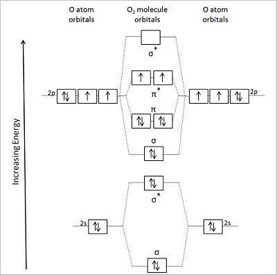
(CC) Image: Anthony.Sebastian Diagrammatic representation of the molecular orbitals of an oxygen molecule (center) formed by the overlapping valence shell orbitals of two flanking oxygen atoms (left and right of center. Asterisks designate antibonding orbitals.
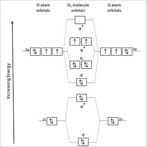
(CC) Image: Anthony.Sebastian Diagrammatic representation of the molecular orbitals of an oxygen molecule (center) formed by the overlapping valence shell orbitals of two flanking oxygen atoms (left and right of center. Asterisks designate antibonding orbitals.
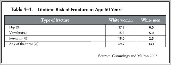
Risks of Developing Osteoporosis in Women and Men
Fractures, a common consequence of osteoporosis, and often the first indication of the disease, rank as osteoporosis' most adverse consequence. It of causes severe pain and debilitation, especially in the elderly who fall and fracture their hip, and it can lead to death from complications during the planned recovery period. Some 20% of hip fracture patients die within a year (Leibson et al. 2002).
The 1.5 million osteoporotic fractures in the United States each year lead to more than half a million hospitalizations, over 800,000 emergency room encounters, more than 2,600,000 physician office visits, and the placement of nearly 180,000 individuals into nursing homes. Hip fractures are by far the most devastating type of fracture, accounting for about 300,000 hospitalizations each year (Surgeon General 2004).
The accompanying table from the Surgeon General's 2004 report (Surgeon General 2004) indicates that at age 50 years white women carry a lifetime risk of hip, spine or forearm fracture amounting to nearly 40%, and men about 13%.
Surgeon General Report on Bone Health and Osteoporosis in 2004 (Surgeon General 2004).
The gender difference relates in part to the faster waning of sex steroid hormones in women as they age, menopause predating the more gradual andropause. Male and female sex hormones act on bone in a positive way, not surprisingly since successful reproduction depends in many ways on healthy bones in the parents.
References Cited
- Listed here in alphabetical order by last name of first author as cited with publication date in the text.
- Leibson CL, Tosteson AN, Gabriel SE, Ransom JE, Melton LJ. (2002) Mortality, disability, and nursing home use for persons with and without hip fracture: a population-based study. J Am Geriatr. Soc. 50(10):1644-50. PMID 12366617.
- Abstract: OBJECTIVES: To compare persons with and without hip fracture for subsequent mortality and change in disability and nursing home (NH) use. DESIGN: Population-based historical cohort study. SETTING: Olmsted County, Minnesota. PARTICIPANTS: All residents who experienced a first hip fracture between January 1, 1989, and December 31, 1993, and, for each case, a resident of the same sex and similar age who had not experienced a hip fracture and was seen by a local care provider. MEASUREMENTS: Data on disability (Rankin score), comorbidity (Charlson Index), and NH residency before baseline (fracture date for cases and registration date for controls) were obtained by review of complete community-based medical records. The records were then reviewed from baseline through December 31, 1994, for Rankin disability at 1 month and 1 year, all NH admissions and discharges, and date of death for those who died. RESULTS: There were 312 cases and 312 controls (81% female, mean age +/- standard deviation = 81 +/- 12 years). Before baseline, cases had higher comorbidity (45% vs 30% had Charlson Index >/= 1, P <.001) and disability (mean Rankin score = 2.5 +/- 1.1 vs 2.2 +/- 1.1, P <.001) and were more likely to be in a NH (28% vs 18%, P <.001) than controls. One year after baseline, estimated mortality was 20% (95% confidence interval (CI) = 16-24) for cases vs 11% (95% CI = 8-15) for controls, 51% of cases versus 16% of controls had a level of disability one or more units worse than before baseline (P <.001), and the cumulative incidence of first NH admission was 64% (95% CI = 58-71) for cases versus 7% (95% CI = 4-11) for controls. The risk of NH admission for cases relative to controls diminished over time, but remained elevated 5 years after the event (risk ratio = 20.0 at 3 months and 2.1 at 5 years), but, in persons admitted to a nursing home, cases were two times more likely than controls to be discharged alive within a year (P <.001). CONCLUSIONS: Hip fracture is an important contributor to disability and NH use, but the potential savings from hip fracture prophylaxis may be overestimated by studies that fail to consider differential risk, mortality, and long-term follow-up.
- Cummings SR, Melton LJ. (2002) Epidemiology and outcomes of osteoporotic fractures. Lancet 359(9319):1761-7 PMID 12049882.
- Abstract: Bone mass declines and the risk of fractures increases as people age, especially as women pass through the menopause. Hip fractures, the most serious outcome of osteoporosis, are becoming more frequent than before because the world's population is ageing and because the frequency of hip fractures is increasing by 1-3% per year in most areas of the world. Rates of hip fracture vary more widely from region to region than does the prevalence of vertebral fractures. Low bone density and previous fractures are risk factors for almost all types of fracture, but each type of fracture also has its own unique risk factors. Prevention of fractures with drugs could potentially be as expensive as medical treatment of fractures. Therefore, epidemiological research should be done and used to identify individuals at high-risk of disabling fractures, thereby allowing careful allocation of expensive treatments to individuals most in need.
Scientists
For biographies of scientists.
Template:Infobox Scientist
Table from OO
| DATE
|
EVENTS PERTINENT TO THE LIFE, WORK AND TIMES OF J.B.S. HALDANE
|
|
|
|
| 1837-1901
|
The Victorian Age: Reign of Victoria, Queen of England and Ireland
|
| 1859
|
Charles Darwin publishes On the Origin of Species, or the Preservation of Favoured Races in the Struggle for Survival.
|
| 1866
|
Gregor Mendel ...
|
| 1892
|
J.B.S. Born, November 5, John Burdon Sanderson Haldane, Oxford, England
|
| ~1894
|
J.B.S. states: "I suppose my scientific career began at the age of about two, when I used to play on the floor of his laboratory and watch him playing a complicated game called "experiments"-the rules I did not understand, but he clearly enjoyed it." [1]
|
| 1896
|
Birth of J.B.S.'s sister, Naomi; later becomes Lady Mitichison
|
| 1900
|
Rediscovery of Gregor Mendel’s Laws of Heredity by Carl Correns, Erik von Tschermak, and Hugo de Vries; those works later to occupy JBS in attempting to synthesize Mendel's Laws and Darwin's theory of evolution.
|
| ~1900-1906
|
J.B.S. states: "At the age of eight or so I was allowed to take down numbers which I called out when reading the burette of a gas-analysis apparatus and later to calculate from these numbers the amounts of various gases in a sample. After this I was promoted to making up simple mixtures for his use and, still later, to cleaning apparatus." [1]
|
| ~1901
|
At age 8 years, J.B.S. accompanies his father to attend a lecture by the British experimental geneticist, Arthur Dukinfield Darbishire (1879–1915), reportedly on Mendel’s laws of inheritance, but possibly also on an opposing view of heredity, given Darbishire’s years of work attempting to reconcile the two views, the biometric and Mendelian views. [2]
|
| ~1904+
|
J.B.S. states: "After I was twelve, he [J.B.S.'s father] discussed with me all his research before publication, and sometimes tried out a lecture course on me before delivering it to students." [1]
|
| 1912
|
J.B.S. at age 19 or 20, publishes his first scientific paper, on human respiratory physiology, co-authored with his father J.S. Haldane and his father’s collaborator, C.G. Douglas.
|
|
|
|
|
|
|
|
|
|
|
|
|
|
|
|
|
|
|
|
|
|
|
|
|
|
|
|
|
|
|
|
|
|
|
|
|
|
|
|
|
|
|
|
|
|
|
|
|
|
|
|
|
|
|
|
|
|
|
|
|
|
|
|
|
|
|
|
|
|
|
|
|
|
|
|
|
|
|
|
|
|
|
|
|
|
|
|
|
|
|
|
|
|
|
|
|
|
|
|
|
|
|
|
|
|
|
|
|
|
|
|
|
|
|
|
|
|
|
|
|
|
|
|
|
|
|
|
|
|
|
|
|
|
|
|
|
|
|
|
|
|
|
|
|
|
|
|
|
|
|
|
|
|
|
|
|
|
|
|
|
|
|
|
|
|
|
|
|
|
|
|
|
|
|
|
|
|
|
|
|
|
|
|
|
|
|
|
|
|
|
|
|
|
|
|
|
|
TIMETABLE OF EVENTS PERTINENT TO THE LIFE, WORK AND TIMES OF J. B. S. HALDANE (referred in this chronology as J.B.S.)
| Year(s)
|
Event
|
| 1837-1901
|
The Victorian Age: Reign of Victoria, Queen of England and Ireland.
|
| 1892
|
John Burdon Sanderson Haldane (J. B. S. Haldane) born, month-day, Oxford, England
|
| ~1894
|
J.B.S. states: “I suppose my scientific career began at the age of about two, when I used to play on the floor of his laboratory and watch him playing a complicated game called "experiments"-the rules I did not understand, but he clearly enjoyed it.”[1]
|
| 1896
|
Sister Naomi born; later known as Lady Mitchison
|
| 1900
|
Rediscovery of Gregor Mendel’s Laws of Heredity by Carl Correns, Erik von Tschermak, and Hugo de Vries
|
| ~1900-1906
|
J.B.S. states: “At the age of eight or so I was allowed to take down numbers which I called out when reading the burette of a gas-analysis apparatus and later to calculate from these numbers the amounts of various gases in a sample. After this I was promoted to making up . simple mixtures for his use and, still later, to cleaning apparatus.”[1]
|
| ~1901
|
At age 8 years, J.B.S. accompanies his father to attend a lecture by the British experimental geneticist, Arthur Dukinfield Darbishire (1879–1915), reportedly on Mendel’s laws of inheritance, but possibly also on an opposing view of heredity, given Darbishire’s years of work attempting to reconcile the two views, the biometric and Mendelian views.[3]
|
| ~1904+
|
J.B.S. states: “After I was twelve, he discussed with me all his research before publication, and sometimes tried out a lecture course on me before delivering it to students.” .”[1]
|
| 1912
|
J.B.S.’s first scientific paper published, on human respiratory physiology, co-authored with his father J.S. Haldane and his father’s collaborator, C.G. Douglas.
|
|
|
|
|
|
|
|
|
|
|
|
|
|
|
|
|
|
|
|
|
|
|
|
|
|
|
|
|
|
|
|
|
|
|
|
|
|
|
|
|
|
|
|
|
|
|
|
|
|
|
|
|
|
|
|
|
|
|
|
|
|
|
|
|
|
|
|
|
|
|
|
|
|
|
|
|
|
|
|
|
|
|
|
|
|
|
|
|
|
|
|
|
|
|
|
|
|
|
|
|
|
|
|
|
|
|
|
|
|
|
|
|
|
|
|
|
|
|
|
|
|
|
|
|
|
|
|
|
|
|
|
|
|
|
|
|
|
|
|
|
| Year(s)
|
Event
|
| 1837-1901
|
The Victorian Age: Reign of Victoria, Queen of England and Ireland.
|
| 1892
|
John Burdon Sanderson Haldane born, month-day, Oxford, England
|
| 1896
|
Sister Naomi born; later known as Lady Mitchison
|
| 1900
|
Rediscovery of Gregor Mendel’s Laws of Heredity by….
|
|
|
|
|
|
|
|
|
|
|
|
|
|
|
|
|
|
|
|
|
|
|
|
|
|
|
|
|
|
|
|
|
|
|
|
|
|
|
|
|
|
|
|
|
|
|
|
|
|
|
|
|
|
|
|
|
|
|
|
|
|
|
|
|
|
|
|
|
|
|
|
|
|
|
|
|
|
|
|
|
|
|
|
|
|
|
|
|
|
|
|
|
|
|
|
|
|
|
|
|
|
|
|
|
|
|
|
|
|
|
|
|
|
|
|
|
|
|
|
|
|
|
|
|
|
|
|
|
|
|
|
|
|
|
|
|
|
|
|
|
|
|
|
|
|
|
|
|
|
|
|
|
|
|
|
new table
| Shell #
|
Subshell
Number
|
No. of
Orbitals
|
Orbital
Type
|
Orbital
Label
|
| 1
|
0
|
1
|
1s
|
s
|
| 2
|
0
1
|
1
3
|
2s
2p
|
s
px, py, p
|
| 3
|
0
1
2
|
1
3
5
|
3s
3p
3d
|
s
px, py, p
dxy, dxy, dyz, dx2-y2, dz2
|
| 4
|
0
1
2
3
|
1
3
5
7
|
4s
4p
4d
4f
|
s
px, py, p
dxy, dxy, dyz, dx2-y2, dz2
See f orbitals here
|
|
|
|
table
| Shell #
|
Subshell
Number
|
No. of
Orbitals
|
Orbital
Designation
|
| 1
|
0
|
1
|
1s
|
| 2
|
0
1
|
1
3
|
2s
2p
|
| 3
|
0
1
2
|
1
3
5
|
3s
3p
3d
|
| 4
|
0
1
2
3
|
1
3
5
7
|
4s
4p
4d
4f
|
|
|
|
Atomic orbital tbl
| Table: Features of Atomic Structure in Relation to Orbitals
|
| Shell #
n
|
Subshell
Number
l
|
Number of
Orbitals in
Subshell
|
Orbital Type
(Subshell Notation)
|
Number of Orbitals
per Subshell
|
Orbital Label
|
Number of Electrons
Needed to Fill Subshell
|
Total Number of
Electrons in Subshell
|
| 1
|
0
|
1
|
1s
|
1
|
1s
|
2
|
2
|
| 2
|
0
1
|
1
3
|
2s
2p
|
1
3
|
2s
2px 2py 2pz
|
2
6
|
8
|
| 3
|
0
1
2
|
1
3
5
|
3s
3p
3d
|
1
3
5
|
3s
3px 3py 3pz
3dxy 3dxz 3dyz 3dx2y2 3dx2
|
2
6
10
|
18
|
| 4
|
0
1
2
3
|
1
3
5
7
|
4s
4p
4d
4f
|
1
3
5
7
|
4s
4px 4py 4pz
4dxy 4dxz 4dyz 4dx2-y2 4dz2
See f orbital labels here
|
2
6
10
14
|
32
|
| n = the principal quantum number, designating shell #s of increasing energy levels as more energy must be absorbed to maintain electrons more distant from the positively charged nucleus; l = the angular momentum of the orbitals segregating them into subshells numbered as l, which increases monotonically.
|
|
|
References
Citations and Notes
|
|


